So I've been working on this project at work lately trying to optimize deliveries to customers that involves a lot of geospatial analysis and computation of driving distances and times. We thought it would be a good idea to write up a blog post about the tools we're using to do this analysis (and I will probably write another post about the project itself later), so here it is.

This is a slight modification of the original post, which you can find on ATD's Medium blog. You can find Part 1 here, and here is Part 2. (This post here is a combo of both; I couldn't wait). Unfortunately for Medium, they don't allow interactive HTML elements (or the use of Markdown at all!), and I wanted to show off all the cool interactive visualizations that you can make by using folium/leaflet.js, which I can do here on my blog, since I like... own the website.

Motivation

At ATD, we make a lot of deliveries to our customers. Every year, our delivery fleet cumulatively drives roughly 90 million miles, making 7 million deliveries to customers on one of the 650 thousand delivery trips we make.

That's a lot of ground to cover, and so anything that we can do to reduce the distance we drive (and therefore our carbon footprint) is a good idea.

As part of our last-mile delivery service, we orchestrate all our deliveries through some 3rd-party software. It does very well, but there are certain cases where we want to modify the routes it suggests to try and improve our delivery efficiency. For this reason, we often find ourselves analyzing delivery routes from a geospatial and routing perspective.

Driving vs "straight-line" distances

It is very important that distances between stops are taken into account accurately, because if we were to use the "straight-line" (aka "great circle", "as the crow flies", "haversine", etc.) distance between two points on the globe, you could potentially vastly underestimate the actual distance that a vehicle would have to drive between those points. A study from the NY State Cancer Registry and U. of Albany (interesting source for a study on driving distances!) found that on average, the actual driving distance between two points is roughly 40% higher than what you would get if you used the "straight-line" distance, which can greatly influence your analysis!

So how do you get this information? Well, you could look it up on Google Maps, but that would be incredibly tedious to go through all the stops one by one, type it into the browser... ugh. Fortunately Google Maps has an API that you can use to programattically request this data using your language of choice. This makes it very easy just get the data and forget about how it was generated.

However, if you look at Google's pricing information, you'll see that this ease comes with a pretty hefty cost. If you have 500 locations that you want to find the distance (or time) matrix for, that will cost you about (500^2 requests) * ($5/1000 requests) = $1250. This is a one-time expense (as long as the locations don't change, or new/old roads get opened/closed), but what do you do if you have to scale up or don't have the budget? ATD has roughly 70,000 active customers; we don't want to spend tens of thousands of dollars acquiring this data! Or what if you're Amazon and deliver to MILLIONS of unique customers? Or maybe you're just a college student who can't afford to spend hundreds of dollars just to analyze a small dataset for fun?

If only there was an open source version of the Google Maps API that you could run for free (or at least significantly cheaper)...

OSRM to the rescue

You may have heard of OpenStreetMap; it's basically a free, open-source version of Google Maps, where the maps are maintained and updated by an army of dedicated volunteers. It has some basic routing capabilities that you can use manually, and an API, but it's mostly focused on maintaining the maps rather than extracting and analyzing data from them. Enter OSRM (Open Source Routing Machine) - an open source software solution built on top of OpenStreetMap's map data that is capable of calculating routes between locations on the fly, and very quickly too. In a nutshell, it's your own personal version of Google Maps API. You set up a server which accepts HTTP requests containing the location information of the stops, and it returns some data depending on what kind of answer you're asking for (there are many services available, like distance matrix, fastest route, nearest road, etc).

Installation/setup

So first, we have to set up the server. It's kind of an involved process, but if you're willing to spend an afternoon downloading map files and setting up docker containers in exchange for saving a bunch of money, I think it's a good tradeoff.

First off, the requirements for installation: depending on the region(s) you want to analyze, you will need roughly 30 MB (for Antarctica) to 50 GB (for the whole planet) of disk space for the map files, about 7-8 times as much more for all the pre-processing files (so 8-9x map size in total), and then RAM requirements (for installation) are roughly 10 times as much as the map size. After installation, the RAM needed to run the software is only 3-5 times as much as the file size for the map. (So if my map is 9 GB, I probably need at least 80 GB of disk space, and 90 GB of RAM for installation, and then only about 30-40 GB of RAM when running the server after installation.)

This may be too much for a single machine to handle, especially if you're just a data enthusiast working on a laptop. But don't stop reading yet! There are cheap and abundant cloud computing resources that were made for just this purpose. For this scenario, I'm going to use Google Cloud Platform (GCP). If you sign up for a new account, they'll give you a $300 credit too, which is more than enough to cover the compute costs. I'll walk you through it if you don't already have a GCP account set up. Go ahead and skip this part if you already have a cloud provider or want to use your own machine.

Google Cloud setup

Go to https://cloud.google.com/gcp/, sign up for the free trial (it'll ask you for your credit card, but you won't be billed unless you burn through all your free credits), then go to Compute Engine > VM Instances. It'll take a minute to boot up the first time, but once it's done, click "Create" to make a new instance. You'll see an image like the one below

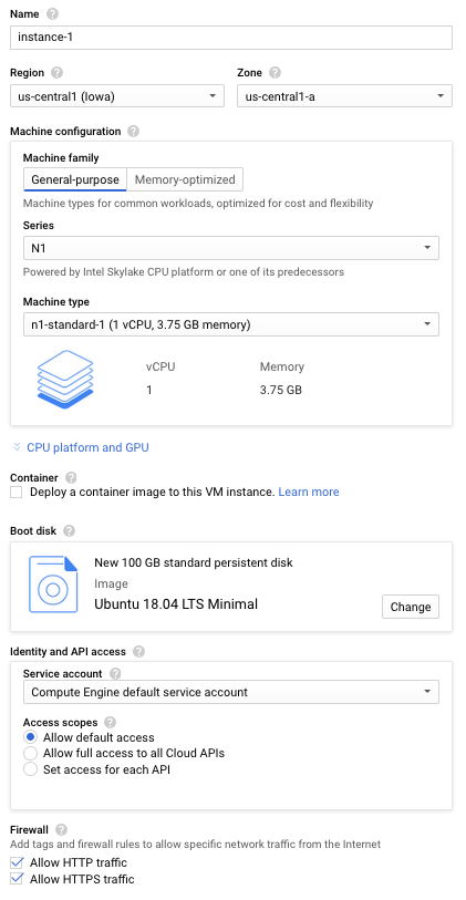
The only thing you really need to make sure of is that you have enough persistent disk space to hold both the map files and all the files created during the pre-processing step, and the machine allows HTTP traffic so that we can make requests against the OSRM server from our local machine. When you check the "allow HTTP traffic" it will allow you to make requests against the server through port 80 (and 443 for HTTPS). I started off with 50 GB of disk space and it turns out that wasn't enough, and I had to resize it to 100 GB after the pre-processing crashed. Don't worry about the RAM right now because we're just going to be downloading files and installing other packages first. I'm pretty familiar with Ubuntu 18.04, so I'll use that, but it shouldn't matter if you want to use a different OS.

We will need to SSH into the machine using the terminal. You can find the command to use by clicking on the dropdown under the "Connect" column and clicking "SSH > view gcloud command" in your "VM Instances" page. You will probably have to log into your GCP account first using

gcloud auth login <your account username>

which will open a series of browser windows you need to click through. You may also have to grant editor privleges to your sevice account before starting the machine. You need to set your current project, whose id you can find from the GCP console by clicking on the dropdown in the upper left corner: . Use that in the following command:

gcloud config set project <your project id>

Now boot up the machine (if it isn't already running) and ssh in (I'd make an alias for these commands too in your .bashrc; you'll be using them a lot):

gcloud compute instances start <instance name> --zone <compute zone>
gcloud beta compute --project "<project id>" ssh --zone "<zone>" "<instance name>"

Alright, you're in! This is a fresh machine, so it probably doesn't have some of the stuff we'll need, like docker or python3, so make sure those are installed properly too before proceeding. [Docker install tutorial]

OSRM setup

The first order of business is to download the map files. You can find a repository of map files at geofabrik.de, which hosts up-to-date versions of OpenStreetMaps data for free. You can download an entire continent at once, or just an individual country/state if you want. (Or you can download the entire planet if you're feeling adventurous.) ATD does business in both the US and Canada, so I'm going to download the entire North America map.

mkdir -p ~/osrm/maps && cd ~/osrm/maps
wget https://download.geofabrik.de/north-america-latest.osm.pbf maps/

This should only take a couple minutes depending on which map you decide to download and your internet connection.

Next we have to get the OSRM backend, which is conveniently packaged into a docker container that's easy to download and run. You can find it at docker hub under the project name osrm/osrm-backend. Simply pull the container file. Do not start the installation just yet!

sudo docker pull osrm/osrm-backend

Perhaps "installation" isn't the best word. What OSRM needs to do is pre-process the map files so that it can make fast lookups at runtime and calculate routes. Running this pre-processing step is very computationally expensive, but once it's done, you never have to do it again unless you want to update your map files. OSRM has two algorithms that it uses to calculate routes, called multi-level Djikstra and contraction hierarchies. We'll be using the latter because it's faster (but less flexible in some cases).

Because this pre-processing is so memory-intensive, we're going to need more RAM. But that's the beauty of cloud computing - if you need more resources, all you need to do is ask for them! First we need to shut down our VM by returning to our local machine and running

gcloud compute instances stop <instance name> --zone <zone>

or simply go to the GCP console, select your instance and click "Stop". In the console, click into your instance's details, hit "Edit", then change your machine configuration to one with more memory. I'm going to use a custom machine type that provides 100 GB of RAM, which is probably just enough to handle the preprocessing for the North America map (I tried it with 60 GB earlier and ran out of memory). Unfortunately, GCP limits new accounts to using 8 vCPU's max, unless you send them a request to increase. I'll just stick with 8, but if you can get more, it'll make the process go faster.

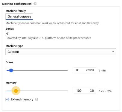
If you're processing a larger map, use more RAM (recall the rule of thumb is 10 times the disk size of the map file). This will be the most "expensive" step, and should cost between $5-$10 depending on how big a machine you're using and how long it runs for. If you're using the $300 credit for a new GCP signup, this won't even make a dent in it. You can handily estimate the cost by using GCP's pricing calculator - change the "Average hours per day each server is running" to "per month" and input the number of hours you think it'll take to do the install. I'd budget at least 10 hours for the North America map, but YMMV.

Now start up your machine with

gcloud compute instances start <instance name> --zone <zone>

and start running the extraction process, which basically takes the raw data from the map file and formats it in a way that OSRM can easily access for calculating routes and whatnot. I don't want to keep the terminal open the whole time the install is running so I'm going to use a pseudo-terminal like tmux so that I can detach and let it run in the background.

tmux new -s osrm
cd ~/osrm/maps
sudo docker run -t -v "${PWD}:/data" osrm/osrm-backend osrm-extract --threads 8 -p /opt/car.lua /data/north-america-latest.osm.pbf

This'll take like an hour to run. During the process, a lot of output will be produced in the terminal. Most of it is just general info about what's happening, prefixed with [info], but some of it will be "warnings" and prefixed with [warn]. You'll probably get a bunch of warnings regarding u-turns... that's totally normal, so don't worry about it. If you run out of memory (like I did before I increased my RAM to 100 GB), you'll get an error like this:

[error] [exception] std::bad_alloc
[error] Please provide more memory or consider using a larger swapfile

If you ran this in tmux, then just press Ctrl+B followed by D to "detach" the terminal. Then you can go do whatever else you want, and when you want to check back in on the extraction process, simply re-attach the terminal with

tmux a -t osrm

After that's complete, you'll see that there a bunch of new files in the ~/osrm/maps/ directory that were produced during the extraction process. Finally, start the contraction hierarchy pre-processing by running

sudo docker run -t -v "${PWD}:/data" osrm/osrm-backend osrm-contract --thread 8 /data/north-america-latest.osrm

This one will take several hours to run, so go watch a movie, or run it overnight and come back in the morning. If you get some error, it's probably because you don't have enough RAM, so you'll need to resize your VM and try again. You'll probably also get several [warning]s during the process; these are most likely harmless, so don't worry about them.

Once this final step is done, shut down your VM as soon as you can to avoid having to pay any more for using large amounts of RAM; from now on, we won't need as much to run the server. I was able to get away with using 30 GB of RAM for the north-america-latest map. You can check your memory usage by running free -h in the terminal.

Using OSRM from the terminal/browser

So now that the pre-processing step is done, we can finally start the OSRM server and interact with it. Run the following command to boot up the server:

sudo docker run -d -p 80:5000 --rm --name osrm -v "${PWD}:/data" osrm/osrm-backend osrm-routed --max-table-size 1000 --algorithm ch /data/north-america-latest.osrm

Let me briefly break this down:

sudo docker run     # run a docker image
-d      # run in "detached" mode so the terminal output doesn't clutter the screen
-p 80:5000    # publish the container port (5000) to the host port (80) so the container can communicate with the "outside world". Remember when we were saying to check the "allow HTTP traffic" box earlier?
--rm    # delete the container after exit
--name osrm     # name the container "osrm"
-v "${PWD}:/data"       # Create a filesystem internal to the container with the directory structure "/data" which maps the current VM directory to the container's
osrm/osrm-backend       # the name of the docker image
osrm-routed     # start the OSRM server
--max-table-size 1000       # set max allowed distance matrix size to 1000x1000 locations
--algorithm ch      # use the contraction hierarchies algorithm
/data/north-america-latest.osrm     # use the map file we put in the /data directory

Once it starts (run sudo docker logs -f osrm to view the output; it'll print out some stuff like "starting engines... threads... IP address/port..."; when it says [info] running and waiting for requests, go ahead and Ctrl+C to stop following the logs... or keep following them, up to you) we can go ahead and make requests against the server. For example:

curl "http://localhost:80/route/v1/driving/-80.868670,35.388501;-80.974886,35.236367?steps=true"

Refer to the documentation for the finer details on how to structure your request; there are also examples on the right-hand side of the page. We'll also discuss this a bit more in the python section below. Running the above command in the terminal on your VM should return a JSON payload containing all the turn-by-turn details of how to get from the first set of coordinates to the second. (In this JSON will be a polyline encoding that looks like a garbled mess of characters; you can decode this by pasting it into Google Map's interactive polyline utility.) If you replace localhost with your external IP, then you can directly paste the URL into the browser window on your local machine and see the same output (probably formatted a bit nicer too). All you need to do is replace router.project-osrm.org in the examples with the domain name of your server, which is localhost:80 if you're executing this on the VM, or if you want to send requests to the VM from your local machine, you need to look up the "external IP" for the VM in the cloud console. Actually, 80 is a special port - you don't even need to include it when making requests because it's the default HTTP port - but I'll keep using it for completeness' sake. If you want to use a different port for your own purposes, you'll have to adjust your GCP firewall rules to allow traffic to connect through the port.

Also, be warned, the VM's external IP changes every time you start/stop your machine! You can either look this up manually from the GCP console every time, or you can script it using the command

export EXTERNAL_IP=$(gcloud compute instances describe $INSTANCE_NAME --zone=$GCP_ZONE --format='get(networkInterfaces[0].accessConfigs[0].natIP)')

so that you can easily access it through an environment variable such as echo $EXTERNAL_IP. (INSTANCE_NAME and GCP_ZONE will have to be defined in order for this to work.)

If you want to shut the server down, all you need to do is sudo docker kill osrm. Since we set the --rm flag, the container will automatically be removed from the list of active containers, and then you can just start it back up again by running that sudo docker run ... command from earlier.

OSRM's services

OSRM provides a number of different services. The route service will basically give you the driving route between a sequence of points, in the order supplied. It won't optimize the order for you, but there is a trip service plugin that can. The nearest service will find the nearest road to the supplied (latitude, longitude) coordinate. The table service will supply you with the distance/time matrices between a set of locations. The match service is similar to the nearest service in that it finds the nearest road to a point, but is more general because it can generate directions along the path defined. The tile service will actually return an image of a section the map, albeit in a "vector tile" format, which contains metadata about the road network.

We'll just be using the route service going forward, but I urge you to check out the other ones; there is some cool stuff you can do with it!

Using OSRM through Python

Now we're going to get into the actual data analysis part! We're going to need some way of interacting with the OSRM server through python. There are already a couple packages out there already to do this for you, notably python-osrm and osrm-py, but we're going to roll our own because it's really not that hard and it will get you more familiar with how the HTTP requests and responses are structured.

To make HTTP requests against our server, we're going to use the python requests package, which makes it easy to handle HTTP and submit requests to the OSRM API. First off, we will need to understand how to structure our requests so that the server will understand them. The OSRM server API takes in requests in the format

GET /{service}/{version}/{profile}/{coordinates}[.{format}]?option=value&option=value

The service is one of the ones mentioned above (route, table, etc.), the version is v1 as of this writing, profile should be something like driving, car, bicycle, or foot. The coordinates are a list of longitude/latitude coordinates separated by semicolons ;. For example, a list of the (latitude, longitude) coordinates (67.891, 12.345), (78.912, -23.456), (89.123, 34.567) would be formatted like:

coordinates = 12.345,67.891;-23.456,78.912;34.567,89.123

We can write a simple python function which will do this for us automatically so we don't have to worry about doing it every time we make a request:

def format_coords(coords: np.ndarray) -> str:
    """
    Formats numpy array of (lat, lon) coordinates into a concatenated string formatted
    for the OSRM server.
    """
    coords = ";".join([f"{lon:f},{lat:f}" for lat, lon in coords])
    return coords

The format string is optional, and there's only one option anyway (json), so we don't need to worry about it. The options are different for every service, but they take the same format. We can format a python dictionary so that it is output in this way using the following function:

def format_options(options: Dict[str, str]) -> str:
    """
    Formats dictionary of additional options to your OSRM request into a
    concatenated string format.
    """
    options = "&".join([f"{k}={v}" for k, v in options.items()])
    return options

Now we want to make a connection to the server and start making requests. I'm going to create a Connection class that will hold the host IP address/port so we don't have to keep manually inputting this data; any subsequent functions we define for interacting with the server will be methods of this class.

class Connection:
    """Interface for connecting to and interacting with OSRM server.
    
    Default units from raw JSON response are in meters for distance and seconds for
    time. I will convert these to miles/hours respectively.
    """
    METERS_PER_MILE = 1609.344
    SEC_PER_HOUR = 3600
    def __init__(self, host: str, port: str):
        self.host = host
        self.port = port

Now we can combine these two functions to create a base method for making any request against the OSRM server, regardless of which service we're using:

def make_request(
        self,
        service: str,
        coords: np.ndarray,
        options: dict=None
    ) -> Dict[str, Any]:
    """
    Forwards your request to the OSRM server and returns a dictionary of the JSON
    response.
    """
    coords = format_coords(coords)
    options = format_options(options) if options else ""
    url = f"http://{self.host}:{self.port}/{service}/v1/car/{coords}?{options}"
    r = requests.get(url)
    return r.json()

This formats our given coordinates and options in the format OSRM expects, then uses the host and port we specified earlier to connect to the server and make a GET request, returning the response in JSON format.

So what can OSRM do for us? Well, we can use it to get the total distance and travel time along a given route (sequence of coordinates). So let's create a method that will use the routing service to request distance and time to travel a given route:

def route_dt(self, coords: np.ndarray):
    """Returns the distance/time to travel a given route.
    """
    x = self.make_request(
        service='route',
        coords=coords,
        options={'steps': 'false', 'overview': 'false'}
    )
    x = x['routes'][0]
    return (x['distance']/self.METERS_PER_MILE, x['duration']/self.SEC_PER_HOUR)

If we could get into the "guts" of the function, we see the JSON object that is returned, x, has multiple pieces, which you can get by using x.keys().

>>> x.keys()
>>> dict_keys(['code', 'routes', 'waypoints'])

The value for code just contains the HTML response code ("Ok" if the response is good). routes contains a list of dictionaries (and only one dictionary in this case since we're requesting one route at a time), where each dictionary has information regarding the route (distance/time, coordinates of intersections along the way, etc), and waypoints has some more location data about the endpoints of the route. The format of the JSON data returned varies depending on what combination of service/options you use, so do some exploring and make sure you understand the response from what you are requesting before you do anything with it.

We would also like visualize the path the delivery routes took. To do that, we can get a polyline associated with the route from OSRM. We can access this by looking at x['routes'][0]['geometry'] from the HTTP response, which gives us a polyline encoded using Google’s Encoded Polyline Algorithm Format. We will need to decode this into a sequence of (lat, lon) pairs, so we will use the polyline package (pip install polyline if you don't already have it). Then we can add a method to our Connection class to handle the request and decoding:

def route_polyline(self, coords: np.ndarray, resolution: str='low'
    ) -> List[Tuple[float, float]]:
    """Returns polyline of route path as a list of (lat, lon) coordinates.
    """
    assert resolution in ('low', 'high')
    if resolution == 'low':
        options = {'overview': 'simplified'}
    elif resolution == 'high':
        options = {'overview': 'full'}
    x = self.make_request(service='route', coords=coords, options=options)
    return polyline.decode(x['routes'][0]['geometry'])

If the overview option is set to simplified, the generated polyline is pretty low-resolution, but we can get a much higher-resolution one by setting it to full. Now that we have all these connection details, we can get started on route visualization!

Analyzing delivery routes

First and foremost, we're going to need some data. I have some data from ATD that you can play around with, containing all the deliveries at our Charlotte distribution center (DC) on November 11, 2019. It's not a big dataset, but enough to get the point across. I've also fuzzed the exact coordinates a little bit in an attempt to anonymize our customers, but they should be fairly close to the real thing. We'll import it using pandas, cast all the data to appropriate types, and take a look:

raw_df = pd.read_csv('delivery_data.csv')
raw_df['arrival_time'] = pd.to_datetime(raw_df['arrival_time'])
raw_df['departure_time'] = pd.to_datetime(raw_df['departure_time'])
raw_df.head()

  route_id   latitude  longitude        arrival_time      departure_time
0        A  35.237665 -81.343199 2019-11-11 12:53:22 2019-11-11 13:10:00
1        A  35.274080 -81.520423 2019-11-11 13:28:46 2019-11-11 13:31:06
2        A  35.286103 -81.540567 2019-11-11 13:45:13 2019-11-11 13:50:48
3        A  35.290060 -81.535398 2019-11-11 13:56:34 2019-11-11 13:59:23
4        A  35.326816 -81.758327 2019-11-11 14:18:30 2019-11-11 14:22:12

So it looks like we have a bunch of delivery stop data. The delivery route is a unique alphanumeric character (A, B, C, ...), and each stop has a (latitude, longitude) coordinate, as well as an arrival and departure time. Just like any good data scientist would, let's do some data cleaning. Why don't we see if there are any null elements in the data?

print(f"Total # rows: {len(raw_df)}")
print("# null elements:")
print(raw_df.isna().sum())

Total # rows: 377
# null elements:
route_id           0
latitude           0
longitude          0
arrival_time      26
departure_time    26
dtype: int64

Looks like there are some null arrival/departure times... what does that mean?

# Take a look at some of the null rows
raw_df[raw_df.isna().any(axis=1)].head(8)

   route_id   latitude  longitude        arrival_time      departure_time
16        A  35.237393 -80.974431 2019-11-11 18:46:11                 NaT
17        A  35.237393 -80.974431                 NaT 2019-11-11 12:00:20
31        B  35.237393 -80.974431 2019-11-11 16:56:57                 NaT
32        B  35.237393 -80.974431                 NaT 2019-11-11 12:24:31
42        C  35.237393 -80.974431 2019-11-11 21:12:11                 NaT
43        C  35.237393 -80.974431                 NaT 2019-11-11 17:02:47
56        D  35.237393 -80.974431 2019-11-11 15:40:38                 NaT
57        D  35.237393 -80.974431                 NaT 2019-11-11 12:33:22

It appears that the null values are associated with the arrival/departure times from the DC itself, which makes sense. There can't be an arrival time at the starting location, and there can't be a departure time from the ending location. If we want to assign a definite visitation order to each location though, we can simply fill in the null values in arrival_time with the non-null values in departure_time, and vice versa, then sort by either one of the times and assign an integer denoting the visitation order (which I'll call seq_num):

# Fill in null values
stops_df = raw_df.copy()
stops_df['arrival_time'].fillna(stops_df['departure_time'], inplace=True)
stops_df['departure_time'].fillna(stops_df['arrival_time'], inplace=True)

# Assign sequence numbers
df = list()
for route_id, group in stops_df.groupby('route_id'):
    group = group.sort_values(by='arrival_time')
    group['seq_num'] = list(range(len(group)))
    df.append(group)
stops_df = pd.concat(df, axis=0)

Great! Now that the data is clean, let's take a look at some summary statistics of the delivery routes. First we'll take a look at the distribution of stop times:

x = stops_df['arrival_time']
x = x.dt.hour + x.dt.minute/60 + x.dt.second/3600
plt.hist(x, bins=20)
plt.title("Distribution of stop arrival times")
locs, _ = plt.xticks()
plt.xticks(locs, [f"{int(h)}:00" for h in locs])
plt.xlabel('Time')
plt.ylabel('Count')
plt.show()

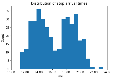
Looks like most of the activity is grouped into two periods - early afternoon and evening deliveries. We can see this more clearly if we look at the initial departure time of each route:

x = stops_df.groupby('route_id')['departure_time'].min()
x = x.dt.hour + x.dt.minute/60 + x.dt.second/3600
plt.hist(x, bins=20)
plt.title("Distribution of initial route departure times")
locs, _ = plt.xticks()
plt.xticks(locs, [f"{int(h)}:00" for h in locs])
plt.xlabel('Time')
plt.ylabel('Count')
plt.show()

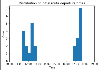
Yep, the routes are definitely separated out into (late morning)/(early afternoon) and late afternoon deliveries. Makes sense, because ATD advertises twice-daily deliveries if you need them. Now how's that for customer service?!

And just how efficient are these delivery stops? Are they quick in-and-out stops with just enough time to drop things off and take off for the next stop, or do we have to hang around and get reciepts signed, find the manager at the location, etc.? We can take the difference between departure times and arrival times and look at that distribution:

x = stops_df['departure_time'] - stops_df['arrival_time']
x = x.dt.seconds/60
x = x[x != 0]   # Filter out "stops" at the distribution center
plt.hist(x, bins=100)
plt.title("Distribution of 'layover' times")
plt.xlabel('Time [minutes]')
plt.ylabel('Count')
plt.show()

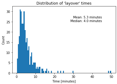
Looks like the vast majority of our stops are pretty efficient! Only 5.3 minutes on average, and half of them are 4 minutes or less! We can only speculate what the outliers may be, but I would guess that they are probably due to issues like the wrong order was shipped, or the driver had to go searching/wait for someone to sign the receipt acknowledging delivery. Either way, these long stop layovers are very rare.

Visualizing delivery routes

Alright, so I promised route visualization and using OSRM in the title; where is it??! Worry no more... Let's start off with simply visualizing the geospatial location of all the customers ATD delivered to on that day. We'll be using the folium package, which provides a nice python API for the leaflet.js mapping utility. The nice thing about leaflet.js is that since it is written in javascript, you can interact with it from within your browser; try it out!

m = folium.Map(location=stops_df[['latitude','longitude']].mean(), zoom_start=8)
for _, row in stops_df.iterrows():
    lat, lon = row['latitude'], row['longitude']
    folium.Marker(
        location=(lat, lon),
        popup=f"({lat:.4f}, {lon:.4f})"
    ).add_to(m)
m

So now, let's start mapping routes. folium has a PolyLine class that we can use to specify the line by passing in a sequence of (lat, lon) coordinates - exactly what we designed our Connection.route_polyline method to return! We'll just focus on a single route for now:

df = stops_df[stops_df['route_id'] == 'A'].copy()
df.sort_values(by='seq_num', inplace=True)
# Create map
m = folium.Map(location=df[['latitude','longitude']].mean(), zoom_start=9)
# Get polyline from OSRM
coords = df[['latitude','longitude']].values
route_polyline = conn.route_polyline(coords, resolution='high')
# Add polyline between stops
folium.PolyLine(
    locations=route_polyline,
    tooltip="Route A",
    color='#0fa6d9',
    opacity=0.75
).add_to(m)
# Create location markers for stops
for _, row in df.iterrows():
    lat, lon = row['latitude'], row['longitude']
    popup = folium.Popup(f"({lat:.4f}, {lon:.4f})", max_width=9999)
    folium.CircleMarker(
        location=(lat, lon),
        popup=popup,
        tooltip=row['seq_num'],
        radius=4,
        fill=True,
        fill_opacity=.25,
        color='#0fa6d9',
    ).add_to(m)
m

That's pretty cool. You can see that the route doesn't really "start" until after the truck passes Gastonia, which is already pretty far away from the distribution center (about 20 miles). If we were to examine all the routes at once, we would see that they are "partitioned", such that some routes deliver to customers who are close to the distribution center, and some routes (like this one) that serve customers who are a bit further away. They each have distinct geographic regions to cover.

You know what, why don't we just map out all the routes? I'll separate them into AM and PM routes - we'll use 14:00 (2pm) as the demarcation between the two, since the route departure times from the histogram we made before look pretty well-separated by that time.

maps = dict()
for key, route_ids in zip(['AM','PM'], [am_route_ids, pm_route_ids]):
    df = stops_df[stops_df['route_id'].isin(route_ids)]
    # Create map
    maps[key] = folium.Map(
        location=df[['latitude','longitude']].mean(),
        zoom_start=8
    )
    # Iterate over route ID's
    for route_id, group in df.groupby('route_id'):
        # Order route stops, choose random color
        group = group.sort_values(by='seq_num')
        color = np.random.choice([
            "#ff0000", # red
            "#ff9500", # orange
            "#ffd900", # yellow
            "#73ff00", # green
            "#00ffd5", # teal
            "#00c3ff", # light blue
            "#0022ff", # dark blue
            "#9d00ff", # purple
            "#ff00ee", # pink
            "#ff00a2", # magenta?
        ])
        # Get polylines from OSRM
        for i in range(len(group)-1):
            coords = group[['latitude','longitude']].values[i:i+2]
            route_polyline = np.array(conn.route_polyline(
                coords, resolution='high'
            ))
            d, t = conn.route_dt(coords)
            # Add polyline between stops
            folium.PolyLine(
                locations=route_polyline,
                tooltip=f"Route {route_id}",
                popup=f"Distance: {d:.2f} mi., duration: {60*t:.1f} min.",
                color=color,
                opacity=0.35,
            ).add_to(maps[key])
        # Create location markers for stops
        for _, row in group.iterrows():
            lat, lon = row['latitude'], row['longitude']
            arrival = row['arrival_time'].strftime("%H:%M")
            departure = row['departure_time'].strftime("%H:%M")
            if row['seq_num'] % (len(group)-1) == 0:
                folium.Marker(
                    location=(lat, lon),
                    tooltip='Charlotte DC',
                    popup=folium.Popup(f"({lat:.4f}, {lon:.4f})", max_width=9999),
                    icon=folium.Icon(color='black', icon='home'),
                ).add_to(maps[key])
            else:
                folium.CircleMarker(
                    location=(lat, lon),
                    tooltip=f"{route_id}-{row['seq_num']}",
                    popup=f"({lat:.4f}, {lon:.4f})\n{arrival}-{departure}",
                    radius=4,
                    fill=True,
                    fill_opacity=.5,
                    color=color,
                ).add_to(maps[key])

AM delivery routes

PM delivery routes

Now we can see the routes in all their glory. There are a couple routes that take mostly the same paths, but at different times, like routes (I,Y), (A,C) and (K,L). Then there are routes that are kind of combinations of other routes. For example, in the AM, we have route R, that hits customers in both Statesville and Salisbury, but in the PM, these customers are split between routes S and T. Similarly, in the PM, we have customers near Lancaster and Rock Hill that are all serviced by route G, but in the AM they are split between routes H and V.

These interactive maps contain a lot of information that you couldn't reasonably put on a static map. For example, hovering over a customer location will give you the route they were visited on and which order they were delivered to. Clicking on the location will give the (lat, lon) coordinates and the arrival-departure times. Hovering over a route polyline will give you the route ID, and clicking will give a popup that tells you the expected distance and time it would take to traverse this leg of the route (as calculated by OSRM).

Conclusion

So just to recap, here's all the things that we learned in this post:

1. How to set up a GCP account and compute instance
2. How to download, setup and install OSRM
3. How to use the python requests package to interact with the OSRM server on a remote machine through HTTP
4. How to analyze delivery routes using geospatial and temporal analysis using pandas
5. How to visualize geospatial data using folium

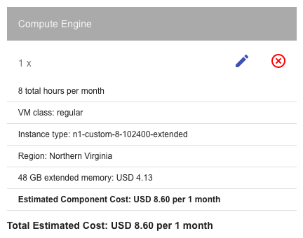
That's a lot of stuff! And we did it all on a pretty tight budget: $0. Just to prove to you that this is not going to break the bank, here's a screenshot of my GCP billing status:

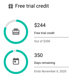
I spent roughly $60 in cloud credits while writing this post, but your costs should be significantly less; the reason mine were so "high" can be attributed to several things:

• I screwed up sizing the RAM on my VM twice before I figured out the right amount and had to run the OSRM pre-computation step multiple times
• I accidentally left the instance on (idling) overnight while it was allocated 100 GB of RAM
• I was lazy and regularly left the VM on while I was writing the blog post, working on other things, or going to get lunch

If you're very efficient and can figure out the right amount of RAM to use to run the OSRM pre-computation the first time, it wouldn't surprise me if you could do all this for less than $10 in cloud credits. Even if your efficiency is terrible, you can get $300 in free credits for just signing up with GCP, so you've got nothing to lose.

I hope you enjoyed following along and learned some helpful analysis techniques. I certainly did too. If you want to see all the code in one place, I have made available a GitHub repository with the jupyter notebook used to generate all the maps, and the dataset used in a .csv format.

© Copyright 2019 by Eric Cotner.

Website generated using Flask / [Source code]